The two-tap scenario with unequal variances

library(rabBITS)
library(tidyverse)
library(patchwork) #for adding ggplots

Two-tap case with unequal variances

In the previous article [REF], we covered the special case where the (inverse) spatial precision, sigma_s is the same for both spatial positions. This is often not realistic, as the spatial resolution of the skin varies between sections of the skin, even along one limb. This can be addressed by a generalized form of the model, that takes single precision parameters for tap 1 and 2.

Prior-Likelihood-Posterior figure with unequal spatial variance

We will create a different version of the figure, where sigma_s1, the inverse precision of tap 1, is 1 and sigma_s2, the inverse precisino of tap 2, takes the value of 2.

Model parameters

The following parameters are used in the article and are used here for plotting.

### Parameters of the stimuli and observer
x1m=3 #measured position of tap 1 (in cm)
x2m=7 #measured position of tap 2 (in cm)
time_t = 0.15 #time between stimuli, i.e., interstimulus time (in seconds)
sigma_s1 = 1 #spatial (im)precision (in cm as a sd)
sigma_s2 = 3 #spatial (im)precision (in cm as a sd)
sigma_v = 10 #low speed prior (in cm/s as an sd)

Parameters for the plots

#params for plots
x1_range <- c(0, 10)
x2_range <- c(0, 10)

#resolution for graphs
x1_res <- 100 
x2_res <- 100

#matrix for the x1-x2 combinations
x1x2Mat <- expand.grid(x1=seq(x1_range[1], x1_range[2], length.out = x1_res), x2=seq(x2_range[1], x2_range[2], length.out = x2_res))

Compute the values for the whole matrix

### XXX Compute prior density
x1x2Mat$prior <- prior_2Tap(x1 = x1x2Mat$x1, x2 = x1x2Mat$x2, time_t = time_t, sigma_v = sigma_v)

### XXX Compute likelihood
x1x2Mat$likelihood <- likelihood_2Tap_UneqVar(x1m=x1m, x2m=x2m, x1=x1x2Mat$x1, x2=x1x2Mat$x2, sigma_s1 = sigma_s1, sigma_s2 = sigma_s2)

### XXX Compute posterior density
x1x2Mat$posterior <- posterior_2Tap_UneqVar(x1m=x1m, x2m=x2m, x1 = x1x2Mat$x1, x2 = x1x2Mat$x2, time_t = time_t, sigma_s1 = sigma_s1, sigma_s2 = sigma_s2, sigma_v = sigma_v)

Create Plots

Now create a plot of all three distributions (like in Figure 2).

#prior
prior.plot <- ggplot(x1x2Mat, aes(x=x1, y=x2, fill=prior)) +
  geom_raster() +
  coord_fixed() +
  ggtitle("prior") +
  theme(legend.position = "none")

#likelihood
likelihood.plot <- ggplot(x1x2Mat, aes(x=x1, y=x2, fill=likelihood)) +
  geom_raster() +
  coord_fixed() +
  ggtitle("likelihood") +
  theme(legend.position = "none")

#posterior
posterior.plot <- ggplot(x1x2Mat, aes(x=x1, y=x2, fill=posterior)) +
  geom_raster() +
  coord_fixed() +
  ggtitle("posterior") +
  theme(legend.position = "none")

Compute posterior modes and add to the plots

We can also add the real positions to the plots and compute the posterior means and add them as well so it becomes better visible how the posterior is dragged towards the prior. The posterior modes are computed with the function posterior_params_2Tap_EqVar()

#likelihood
likelihood.plot <- likelihood.plot +
  geom_point(x=x1m, y=x2m, size=2, color="white", shape=21, fill=NA) #measured position

#posterior modes
Posterior_params <- posterior_params_2Tap_UneqVar(x1m = x1m, x2m = x2m, time_t = time_t,
                                     sigma_s1 = sigma_s1, sigma_s2 = sigma_s2, sigma_v = sigma_v)

Posterior_mode_x1 <- Posterior_params$x1_star
Posterior_mode_x2 <- Posterior_params$x2_star

#update posterior plot
posterior.plot <- posterior.plot +
  geom_point(x=x1m, y=x2m, size=2, color="white", shape=21, fill=NA) + #measured position
  geom_point(x=Posterior_mode_x1 , y=Posterior_mode_x2, size=2, color="red", shape=21, fill=NA) #posterior mode


#join plots
p.joined <- prior.plot + likelihood.plot + posterior.plot
p.joined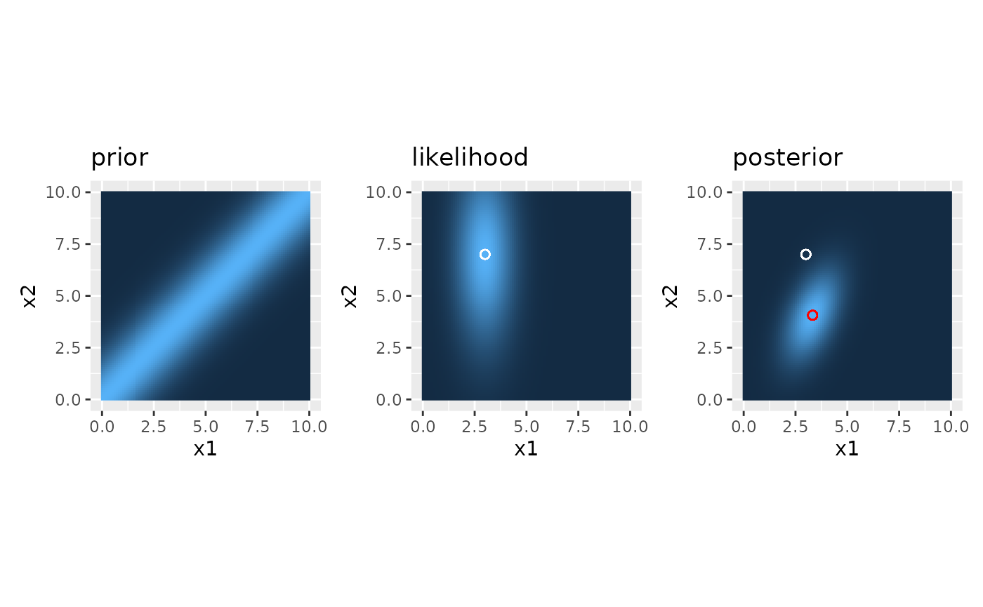

prior, likelihood, and posterior distributions

Numerical sanity check

As a quick sanity check: compare the analytically determined posterior modes to the ones that can be seen in the figure. This can simply be done by finding the value with the highest posterior probability numerically and checking where it is.

#Posterior modes determined analytically
print(paste("analytical values for x1:", 
            round(Posterior_mode_x1, 3),
            "\n and for x2:", 
            round(Posterior_mode_x2, 3)))
#> [1] "analytical values for x1: 3.327 \n and for x2: 4.061"

#Posterior mode determined numerically
posteriorMax <- max(x1x2Mat$posterior)
posteriorMax.index <- which(x1x2Mat$posterior==posteriorMax)

print(paste("numerical values for x1:", 
            round(x1x2Mat$x1[posteriorMax.index], 3),
            "\n and for x2:", 
            round(x1x2Mat$x2[posteriorMax.index], 3)))
#> [1] "numerical values for x1: 3.333 \n and for x2: 4.04"