The two-tap scenario with equal variances
A_two_tap_scenario_equalVariance.RmdTwo-tap case with equal variances
In this simple scenario, we consider two stimuli (“taps”) that are presented on the skin in two positions and are separated in time. The “simple” Bayesian Observer Model makes predictions how the spatiotemporal characteristics of the stimuli, the spatial precisino of the touch sense, and a prior about movement speed influence the perceived positions of the stimuli. In this model, we assume the spatial precision of both touched positions to be idetical, hence it is called the equal variance case.
The used terminology and formulae are based on the article by Goldreich & Tong, 2013, PLOS ONE.
Background information
Some basic assumptions of the Bayesian Observer Model are:
- stimuli (on the skin) are never perceived with perfect precision, because the skin’s spatial resolution is imperfect and therefore each stimulus sensed with a certain (random) measurement error
- successive stimuli are caused by an object moving along the skin
- objects move at a realistic speed. Or, in other words, it is unlikely that objects move very fast and that stimuli therefore move a far distance in a short time
The second assumption is referred to as the low-speed (or: low-velocity) prior.
Hypotheses derived from the model
Some hypotheses that can be derived from the described model are:
- stimuli that are presented far apart and fast will be perceptually attracted towards each other, i.e. there is a perceptual length contraction
- the faster the stimulation, the stronger is the length contraction
- the further the spatial distance between the stimuli, the stronger the length contraction
- the higher the precision, the weaker the length contraction
- the stronger the low-speed prior, the stronger the length contraction
Parameters
The model includes the following parameters:
- \(x_{1m}\) and \(x_{2m}\) as the “measured” or “sensed” positions, i.e. the estimate given by the sensors corresponding to the stimulus positions
- \(x_1\) and \(x_2\) as the inferred or hypothetical stimulus positions
- \(t\) as the time (in seconds) passing between the taps
- \(\sigma_s\) the spatial standard deviation, or uncertainty, referring to the sensed positions (\(x_{1m}\) and \(x_{2m}\)). Higher values indicate lower precision.
- \(\sigma_v\) the degree of the “low-speed” prior. Lower values indicate slower expected speed, or, a “stronger” prior.
A word about units: Although the units of time and space are arbitrary as long as they are consistent, there is a consistent use of units in the literature. Usually, all spatial units \(x_{1m}\), \(x_{2m}\), \(x_1\), \(x_1\), and \(\sigma_s\) are expressed in cm units. And time, \(t\) is expressed as seconds. The low-speed prior \(\sigma_v\) is expressed as space per time units and when using cm and seconds would be cm/s. The \(\sigma_s\) is sometimes conceptually referred to as the average localization error, e.g. with reference to the paper by Weinstein (1968) with 1 cm. Strictly speaking, however, it refers to the standard deviation, or variable error, of spatial localization.
Formula for prior distribution
In the appendix of the article, the formula for the prior distribution is given in Formula A08 as:
\[p(x_1,x_2|t) \propto p(x_2|x_1,t) = \frac {1} {\sqrt{2\pi}\sigma_vt} exp(-\frac {(x_2-x_1)^2}{2(\sigma_v t)^2})\]
Formula for the likelihood distribution
The formula for the likelihood distribution is given in Formula A10 as: \[p(x_{1m},x_{2m}|x_1, x_2, t) = p(x_2|x_1,t) = p(x_{1m}|x_1)*p(x_{2m}|x_2)\] And these two conditional probabilities are defined in A11 as: \[p(x_{1m}|x_1) = \frac {1} {\sqrt{2\pi}\sigma_s} exp \left(-\frac {(x_{1m}-x_1)^2}{2\sigma_s^2} \right)\] and \[p(x_{2m}|x_2) = \frac {1} {\sqrt{2\pi}\sigma_s} exp \left(-\frac {(x_{2m}-x_2)^2}{2\sigma_s^2}\right)\]
Following logically from this, the likelihood computes as: \[p(x_{1m},x_{2m}|x_1, x_2, t) = \frac {1} {\sqrt{2\pi}\sigma_s} exp \left(-\frac {(x_{2m}-x_2)^2}{2\sigma_s^2}\right) * \frac {1} {\sqrt{2\pi}\sigma_s} exp \left(-\frac {(x_{2m}-x_2)^2}{2\sigma_s^2} \right)\]
Formula for the posterior distribution
The formula for the posterior distribution is given in A13 as: \[p(x_1, x_2|x_{1m},x_{2m}, t) \propto exp \left( - \left( \frac {(x_{1m} - x_1)^2 + (x_{2m} - x_2)^2} {2\sigma_s ^2} + \frac {(x_2-x_1)^2}{(2\sigma_v t)^2} \right) \right)\]
The formula for the posterior distribution is also formulated in in A14 as:
\[p(x_1, x_2|x_{1m},x_{2m}, t) \propto exp \left( -\frac {1} {2(1-\rho ^2)} \left( \frac {(x_1 - x_{1*})^2 + (x_2 - x_{2*})^2 - 2 \rho (x_1 - x_{1*}) (x_2 - x_{2*})} {\sigma ^2} \right) \right)\] However, some unknowns appear in this equation which are defined further down in A14. The posterior modes, denoted as \(x_{1*}\) and \(x_{2*}\) are defined as:
\[x_{1*}=x_{1m} \left( \frac {(\sigma_v t)^2 + \sigma_s ^2} {(\sigma_v t)^2 + 2\sigma_s ^2} \right) + x_{2m} \left( \frac {\sigma_s^2} {(\sigma_v t)^2 + 2\sigma_s ^2} \right)\] and: \[x_{2*}=x_{2m} \left( \frac {(\sigma_v t)^2 + \sigma_s ^2} {(\sigma_v t)^2 + 2\sigma_s ^2} \right) + x_{1m} \left( \frac {\sigma_s^2} {(\sigma_v t)^2 + 2\sigma_s ^2} \right)\]
The correlation between the Gaussian distributions \(\rho\) is given as:
\[\rho = \frac {\sigma_s^2} {\sigma_s^2 + (\sigma_v t)^2} \] Finally, the combined variance \(\sigma^2\) is given as:
\[\sigma^2 = \sigma_s^2 \frac {\sigma_s^2 + (\sigma_v t)^2} {2\sigma_s^2 + (\sigma_v t)^2}\]
R implementations of the formulae
Some of the formulae presented above, are implemented in rabBITS:
- Formula A08 is implemented as prior_2Tap()
- Formula A11 is implemented as likelihood_2Tap_EqVar()
- Formula A13 is implemented as posterior_2Tap_EqVar()
- (Parts of) Formula A14 are implemented as posterior_params_2Tap_EqVar()
Note: the R functions presented below can also compute several values at a time, if the parameters are passed as vectors. You will see applications of that in the examples below.
Reproduce Figure 2
In the following, we reproduce Figure 2 from Goldreich & Tong, 2013.
Model parameters
The following parameters are used in the article and are used here for plotting.
### Parameters of the stimuli and observer
x1m=3 #measured position of tap 1 (in cm)
x2m=7 #measured position of tap 2 (in cm)
time_t = 0.15 #time between stimuli, i.e., interstimulus time (in seconds)
sigma_s = 1 #spatial (im)precision (in cm as a sd)
sigma_v = 10 #low speed prior (in cm/s as an sd)
Parameters for the plots
#params for plots
x1_range <- c(0, 10)
x2_range <- c(0, 10)

#resolution for graphs
x1_res <- 100
x2_res <- 100

#matrix for the x1-x2 combinations
x1x2Mat <- expand.grid(x1=seq(x1_range[1], x1_range[2], length.out = x1_res), x2=seq(x2_range[1], x2_range[2], length.out = x2_res))
Compute the values for the whole matrix
### XXX Compute prior density
x1x2Mat$prior <- prior_2Tap(x1 = x1x2Mat$x1, x2 = x1x2Mat$x2, time_t = time_t, sigma_v = sigma_v)

### XXX Compute likelihood
x1x2Mat$likelihood <- likelihood_2Tap_EqVar(x1m=x1m, x2m=x2m, x1=x1x2Mat$x1, x2=x1x2Mat$x2, sigma_s = sigma_s)

### XXX Compute posterior density
x1x2Mat$posterior <- posterior_2Tap_EqVar(x1m=x1m, x2m=x2m, x1 = x1x2Mat$x1, x2 = x1x2Mat$x2, time_t = time_t, sigma_s = sigma_s, sigma_v = sigma_v)
Create Plots
Now create a plot of all three distributions (like in Figure 2).
#prior
prior.plot <- ggplot(x1x2Mat, aes(x=x1, y=x2, fill=prior)) +
  geom_raster() +
  coord_fixed() +
  ggtitle("prior") +
  theme(legend.position = "none")

#likelihood
likelihood.plot <- ggplot(x1x2Mat, aes(x=x1, y=x2, fill=likelihood)) +
  geom_raster() +
  coord_fixed() +
  ggtitle("likelihood") +
  theme(legend.position = "none")

#posterior
posterior.plot <- ggplot(x1x2Mat, aes(x=x1, y=x2, fill=posterior)) +
  geom_raster() +
  coord_fixed() +
  ggtitle("posterior") +
  theme(legend.position = "none")

#join plots
prior.plot + likelihood.plot + posterior.plot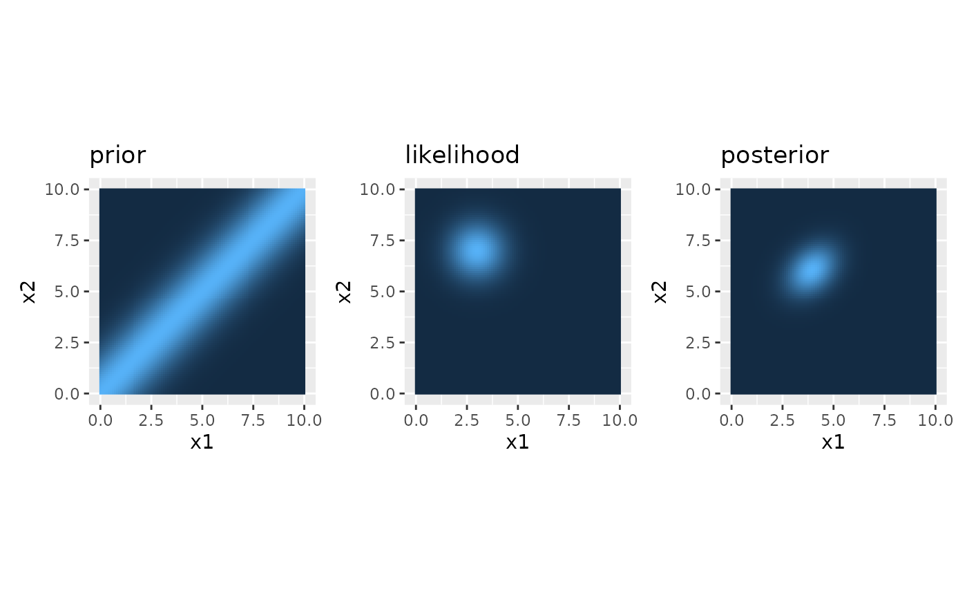
Compute posterior modes and add to the plots
We can also add the real positions to the plots and compute the posterior means and add them as well so it becomes better visible how the posterior is dragged towards the prior. The posterior modes are computed with the function posterior_params_2Tap_EqVar().
#likelihood
likelihood.plot <- likelihood.plot +
  geom_point(x=x1m, y=x2m, size=2, color="white", shape=21, fill=NA) #measured position

#posterior modes
Posterior_params <- posterior_params_2Tap_EqVar(x1m = x1m, x2m = x2m, time_t = time_t,
                                     sigma_s = sigma_s, sigma_v = sigma_v)

Posterior_mode_x1 <- Posterior_params$x1_star
Posterior_mode_x2 <- Posterior_params$x2_star

#version based on A13
posterior.plot <- posterior.plot +
  geom_point(x=x1m, y=x2m, size=2, color="white", shape=21, fill=NA) + #measured position
  geom_point(x=Posterior_mode_x1 , y=Posterior_mode_x2, size=2, color="red", shape=21, fill=NA) #posterior mode


#join plots
p.joined <- prior.plot + likelihood.plot + posterior.plot
p.joined
prior, likelihood, and posterior distributions
The figure looks just like in the article.
Numerical sanity check
As a quick sanity check: compare the analytically determined posterior modes to the ones that can be seen in the figure. This can simply be done by finding the value with the highest posterior probability numerically and checking where it is.
#Posterior modes determined analytically
print(paste("analytical values for x1:",
            round(Posterior_mode_x1, 3),
            "\n and for x2:",
            round(Posterior_mode_x2, 3)))
#> [1] "analytical values for x1: 3.941 \n and for x2: 6.059"

#Posterior mode determined numerically
posteriorMax <- max(x1x2Mat$posterior)
posteriorMax.index <- which(x1x2Mat$posterior==posteriorMax)

print(paste("numerical values for x1:",
            round(x1x2Mat$x1[posteriorMax.index], 3),
            "\n and for x2:",
            round(x1x2Mat$x2[posteriorMax.index], 3)))
#> [1] "numerical values for x1: 3.939 \n and for x2: 6.061"
We can see that the values match quite well.
Addressing the hypotheses
In this section we will evaluate the hypotheses mentioned above by varying model parameters.
Stimuli that are presented far apart and fast will be perceptually attracted towards each other
This hypothesis is inherently confirmed in the computations above: note that the veridical stimuli were presented at positions of 3 and 7 cm, respectively. This is a distance of 4 cm. The posterior modes were at about 3.9 and 6.1 cm. This is only a distance of 2.2 cm. The model accordingly predicts a length contraction of 4 - 2.2 = 1.8 cm for this set of parameters.
The faster the stimulation, the stronger is the length contraction
To address this point, we repeat the model estimations for different values of \(t\), the time passing between the two taps.
modelData <- data.frame(x1m=3, x2m=7, time_t=seq(0, 2, length.out=21), sigma_s=1, sigma_v=10)

#compute posterior modes
modelData$pm_x1 <- with(modelData, posterior_params_2Tap_EqVar(x1m, x2m, time_t, sigma_s, sigma_v))$x1_star
modelData$pm_x2 <- with(modelData, posterior_params_2Tap_EqVar(x1m, x2m, time_t, sigma_s, sigma_v))$x2_star

#create a plot
modelData %>%
  pivot_longer(cols = c(pm_x1, pm_x2), names_to = "posterior", values_to = "position") %>%
  ggplot(aes(x=time_t, y=position, color=posterior)) +
    geom_hline(yintercept = 7, linetype=2, color="grey") +
    geom_hline(yintercept = 3, linetype=2, color="grey") +
    geom_point() +
geom_path() 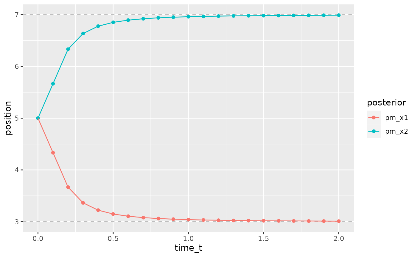
stronger contraction at shorter time t
As can be seen from the figure, the attraction of the stimuli towards each other and the according length contraction is strong for short time intervals between the stimuli and disappears for delays of one second or more.
The further the travelled distance, the stronger the length contraction
To show predictions for this scenario, we keep t and sigma_s constant and vary the positions of the taps. Note that due to the small scale, we have decreased the sigma_s parameter to 0.1 to emphasize the effect.
modelData <- data.frame(x1m=0, x2m=seq(0.1, 1, length.out=10), time_t=0.015, sigma_s=0.1, sigma_v=10)

#compute posterior modes
modelData$pm_x1 <- with(modelData, posterior_params_2Tap_EqVar(x1m, x2m, time_t, sigma_s, sigma_v))$x1_star
modelData$pm_x2 <- with(modelData, posterior_params_2Tap_EqVar(x1m, x2m, time_t, sigma_s, sigma_v))$x2_star

#create a plot
p1 <- modelData %>%
  pivot_longer(cols = c(pm_x1, pm_x2), names_to = "posterior", values_to = "position") %>%
  ggplot(aes(x=x2m, y=position, color=posterior)) +
    geom_abline(intercept = 0, slope = 1, linetype=2, color="grey") +
    xlim(0, 1) + ylim(0, 1) +
    geom_point() +
    geom_path() +
    coord_fixed() +
    ggtitle("posterior modes for \nvarying veridical distances")


#and another plot of the real distance vs. perceived distance
modelData <- modelData %>%
  mutate(veridical=x2m-x1m, perceived=pm_x2-pm_x1) #compute real and perceived distances

p2 <- modelData %>%
  ggplot(aes(x=veridical, y=perceived)) +
  geom_abline(intercept = 0, slope = 1, linetype=2, color="grey") +
  xlim(0, 1) + ylim(0, 1) +
  geom_point() +
  geom_path() +
  coord_fixed() +
  ggtitle("veridical vs. perceived \ndistances")

#merge plots
p1 + p2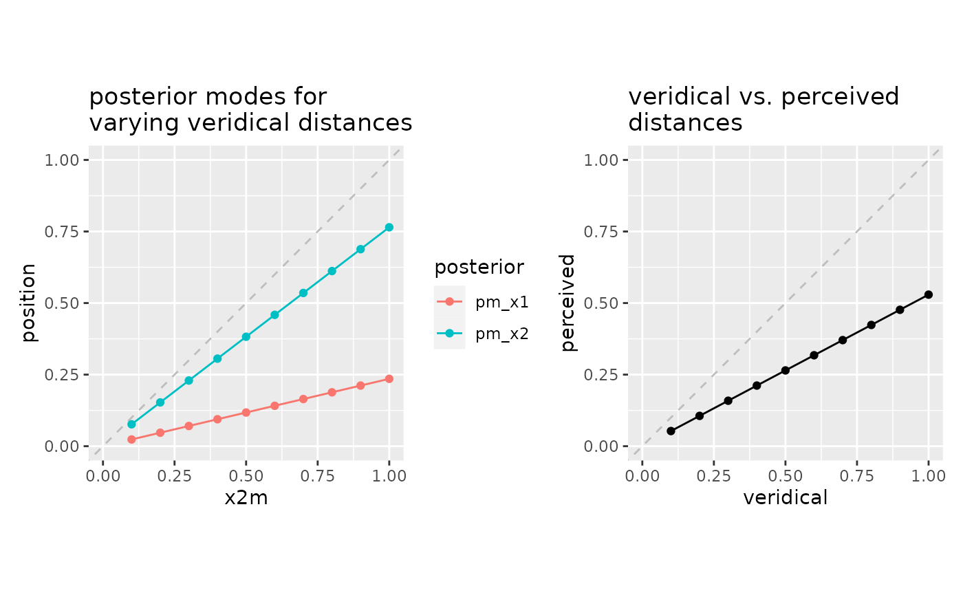
stronger (relative) contraction for larger distances
The higher the precision, the weaker the length contraction
This time we keep parameters all parameters constant except for the sigma_s.
modelData <- data.frame(x1m=3, x2m=7, time_t=0.15, sigma_s=seq(0, 2, length.out=21), sigma_v=10)

#compute posterior modes
modelData$pm_x1 <- with(modelData, posterior_params_2Tap_EqVar(x1m, x2m, time_t, sigma_s, sigma_v))$x1_star
modelData$pm_x2 <- with(modelData, posterior_params_2Tap_EqVar(x1m, x2m, time_t, sigma_s, sigma_v))$x2_star

#create a plot
modelData %>%
  pivot_longer(cols = c(pm_x1, pm_x2), names_to = "posterior", values_to = "position") %>%
    ggplot(aes(x=sigma_s, y=position, color=posterior)) +
    geom_hline(yintercept = 7, linetype=2, color="grey") +
    geom_hline(yintercept = 3, linetype=2, color="grey") +
    geom_point() +
    geom_path() +
    ggtitle("posterior modes for \nvarying spatial precisions")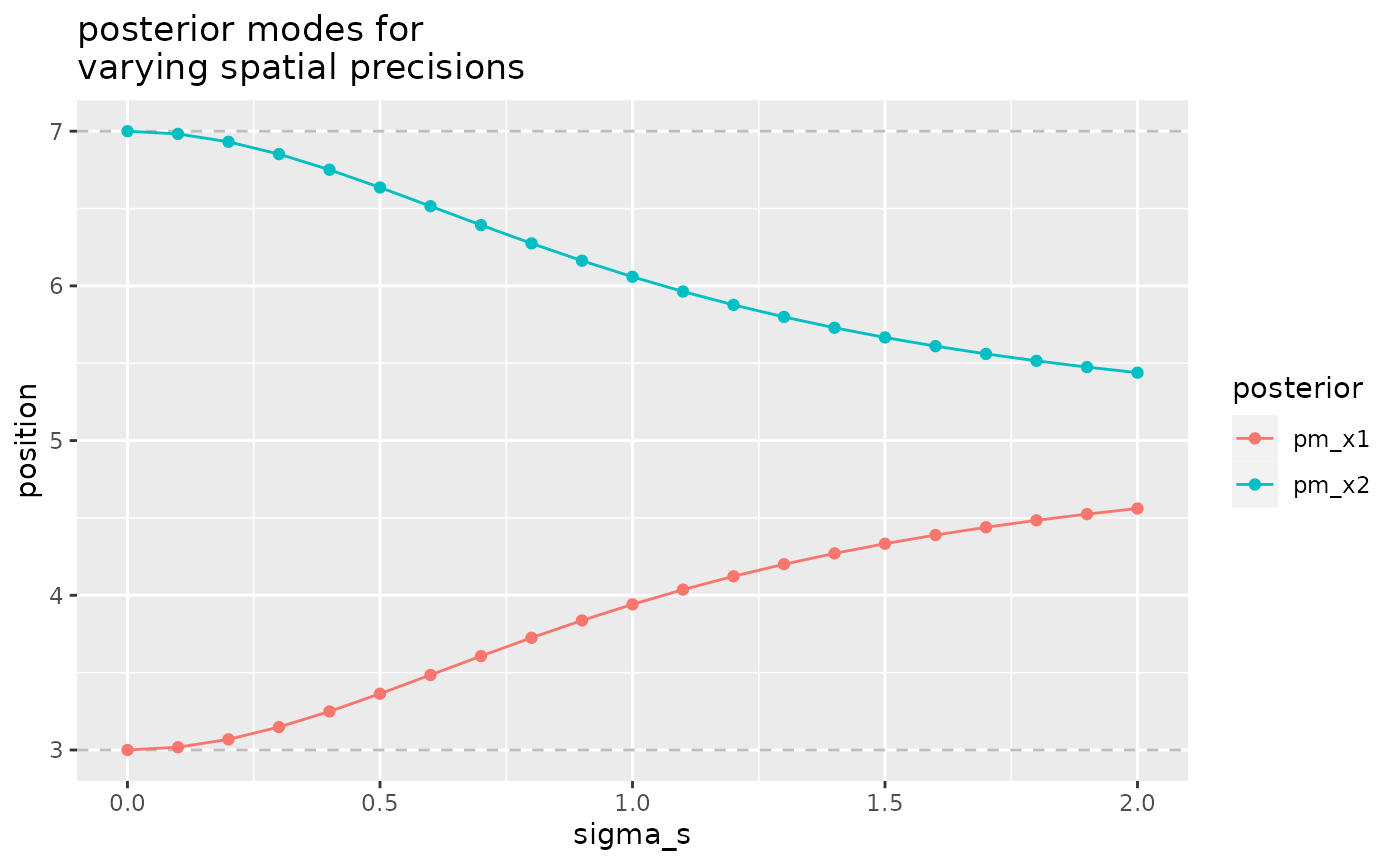
stronger contraction for lower precision
The stronger the low-speed prior, the stronger the length contraction
Finally, the low-speed prior is varied as the only parameter.
modelData <- data.frame(x1m=3, x2m=7, time_t=0.15, sigma_s=1, sigma_v=seq(0, 10, length.out=21))

#compute posterior modes
modelData$pm_x1 <- with(modelData, posterior_params_2Tap_EqVar(x1m, x2m, time_t, sigma_s, sigma_v))$x1_star
modelData$pm_x2 <- with(modelData, posterior_params_2Tap_EqVar(x1m, x2m, time_t, sigma_s, sigma_v))$x2_star

#create a plot
modelData %>%
  pivot_longer(cols = c(pm_x1, pm_x2), names_to = "posterior", values_to = "position") %>%
    ggplot(aes(x=sigma_v, y=position, color=posterior)) +
    geom_hline(yintercept = 7, linetype=2, color="grey") +
    geom_hline(yintercept = 3, linetype=2, color="grey") +
    geom_point() +
    geom_path() +
    ggtitle("posterior modes for \nvarying speed priors")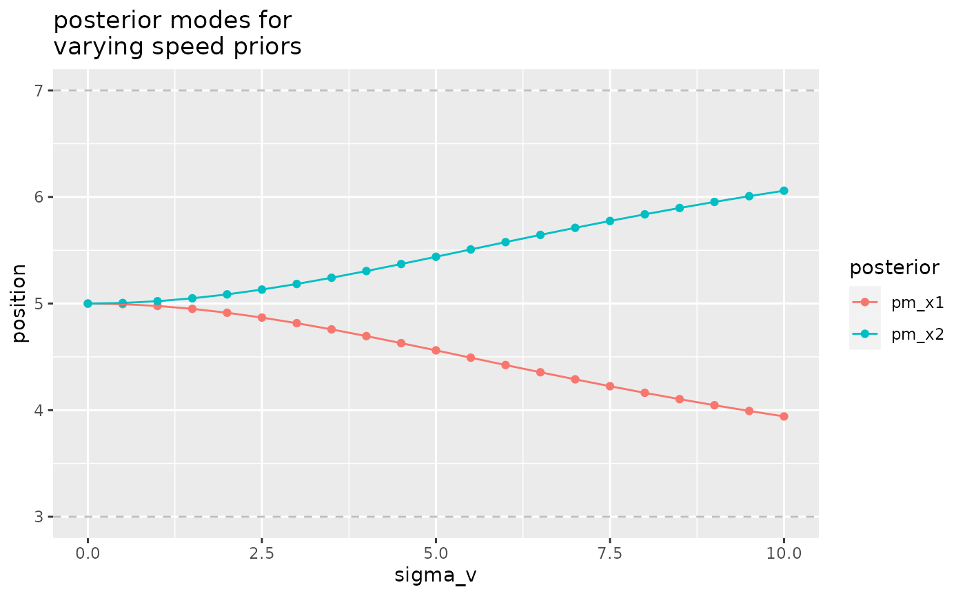
stronger contraction for lower expected speed