Compute posterior probability density for the two-tap scenario with equal spatial variance
posterior_2Tap_EqVar.RdThe function computes values that are proportional to the posterior probability values for the given trajectory. The code refers to the two-tap model with equal variance (spatial uncertainty) for both taps as described in Goldreich & Tong (2013), given in Formula A13.
Arguments
- x1m
measured/sensed or hypothetical position of tap 1 for which the likelihood (p given the other parameters) is computed
- x2m
measured/sensed or hypothetical position of tap 2
- x1
(real) position of tap 1
- x2
(real) position of tap 1
- time_t
speed prior (in units of space per time; given as a standard deviation)
- sigma_s
spatial uncertainty (given as a standard deviation) for the taps (same sd assumed for both positions)
- sigma_v
speed prior (in units of space per time; given as a standard deviation)
Value
values that are proportional to the posterior probability for the given trajectory. If x1 and x2 are vectors, a vector of probabilities is returned. Note that the returned values are not strictly speaking probabilities because they are not normalized (see article for details or the vignette on the two-tap scenario).
Examples
#XXX Example 1: compute a single point estimate XXX
posterior_2Tap_EqVar(x1m=2, x2m=4, x1=2, x2=4, sigma_s=1, sigma_v=10, time_t=0.1)
#> [1] 0.1353353
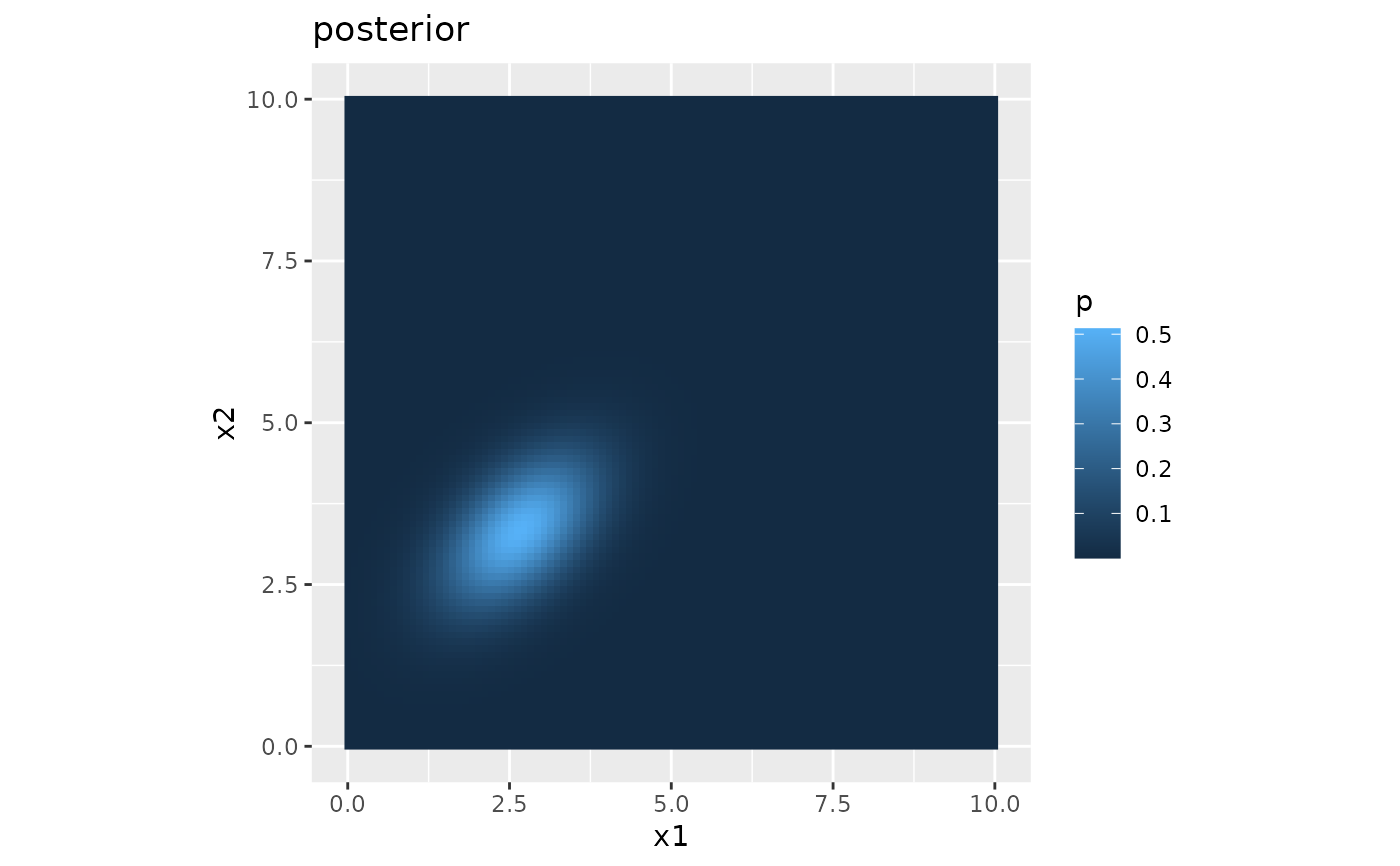
#XXX Example 2: plot a posterior distribution for combinations of tap 1 and 2 XXX
library(ggplot2)
x1_range <- c(0, 10) #range for taps
x2_range <- c(0, 10)
x1_res <- 100 #resolution for graphs
x2_res <- 100
posteriorMat <- expand.grid(x1=seq(x1_range[1], x1_range[2], length.out=x1_res), x2=seq(x2_range[1], x2_range[2], length.out=x2_res))
posteriorMat$p <- posterior_2Tap_EqVar(x1m=2, x2m=4, x1=posteriorMat$x1, x2=posteriorMat$x2, sigma_s=1, sigma_v=10, time_t=0.1)
ggplot(posteriorMat, aes(x=x1, y=x2, fill=p)) +
geom_raster() +
coord_fixed() +
ggtitle("posterior")